Hantush Bierschenk Method

Hantush-Bierschenk (1963) Method

See Also:

The Hantush-Bierschenk method is used to determine linear and non-linear well loss coefficients and to predict drawdown in a well at a specified pumping rate after a specified period of time (delta t).

The method is suitable for confined, leaky, and unconfined aquifers pumped step-wise at increasing rates.

Procedure:

1. Make sure all necessary data has been entered, including a value of delta t from Edit | Aquifer Parameters.

2. Select View | Set Step Drawdowns. Use the control panel to fit best fit lines through each step. It is recommended that early data points from each step be excluded so that the lines have a good fit in the later data points for each step. If the file is saved at this point, the fit of the lines will also be saved.

3. After fitting lines for each step, select View | Hantush-Bierschenk. The values for linear and non-linear well-loss coefficients will be displayed on the graph. An equation describing drawdown in the well at time delta t (entered from Edit | Aquifer Parameters) will also be displayed.

Mathematical Development:

As described by Kruseman and de Ridder, Jacob (1947) developed the following equation to describe drawdown in a pumped well:

Equation 1:

$image\HBEQ1.gif$

where:

B is related to linear well and aquifer loss coefficients

C is the non-linear well loss coefficient

P is equal to 2

Q is the well discharge rate

sw is the drawdown in the well

The Hantush-Bierschenk method is used to determine well efficiency parameters B and C where P = 2. From these values, drawdown in the well at other pumping rates at a fixed time (referred to as delta t in the StepMaster documentation and program) can be determined accounting for linear and non-linear well loss.

Part 1

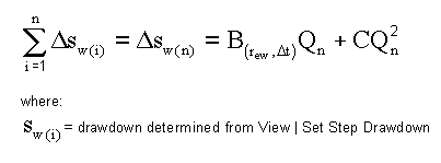
Select View | Set Step Drawdowns. A semi-logarithmic graph of the data points will appear. In the first stage of the procedure, the drawdown Sw for each step is determined. Sw is determined by drawing best fit lines through the data points of each step. Sw is the drawdown difference between each step at time delta t from the beginning of the step. This is shown in the Equation 2.

Equation 2:

$image\HBEQ2.gif$

By rewriting this equation as Equation 3:

Equation 3:

$image\HBEQ3.gif$

This plot is displayed by selecting View | Hantush-Bierschenk.

Part 2

After determining Sw for each step, select View | Hantush-Bierschenk. This will display a graph of Sw/Discharge Rate scaled arithmetically on the vertical axis, and discharge rate scaled arithmetically on the horizontal axis.

The intercept of the line in the vertical axis is the linear well loss coefficient B. A best fit line will be drawn through the points. The slope of the line is the non-linear well loss coefficient C. These values will be displayed over top of the graph.

If the plot of the points is not linear, the assumption that P=2 is not valid, and another method should be used.

An equation describing the drawdown in the well will be displayed under the graph. Data can not be adjusted on the second graph. The first graph should be used for all data adjustments.